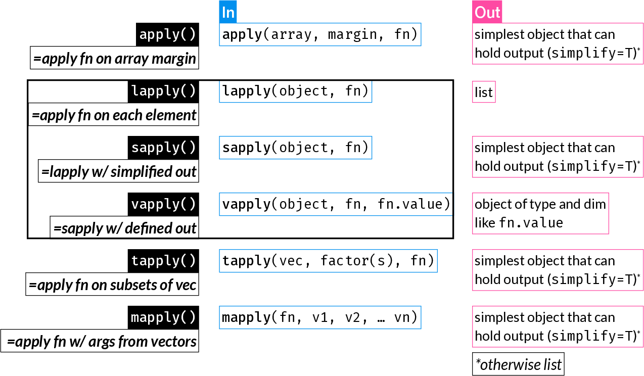
*apply() function family summary (Best to read through this chapter first and then refer back to this figure)
The apply functions are some of the most widely used R functions. They replace longer expressions created with a for loop, for example.
They can result in more compact and readable code.
| Function | Description |
|---|---|
apply() |
Apply function over array margins (i.e. over one or more dimensions) |
lapply() |
Return a list where each element is the result of applying a function to each element of the input |
sapply() |
Same as lapply(), but returns the simplest possible R object (instead of always returning a list) |
vapply() |
Same as sapply(), but with a pre-specified return type: this is safer and may also be faster |
tapply() |
Apply a function to elements of groups defined by a factor |
mapply() |
Multivariate sapply(): Apply a function using the 1st elements of the inputs vectors, then using the 2nd, 3rd, etc. |
*apply() function family summary (Best to read through this chapter first and then refer back to this figure)
apply()
apply() applies a function over one or more dimensions of an array of 2 dimensions or more (this includes matrices) or a data frame:
apply(array, MARGIN, FUN)
MARGIN can be an integer vector or character indicating the dimensions over which ‘FUN’ will be applied.
By convention, rows come first (just like in indexing), therefore:
MARGIN = 1: apply function on each row
MARGIN = 2: apply function on each column
Let’s create an example dataset:
       Age   Weight   Height      SBP
1 38.09655 83.69169 1.680200 133.4053
2 46.08604 65.98232 1.464543 131.9517
3 31.41774 89.68974 1.789754 139.6721
4 40.76269 77.81178 1.886837 136.7120
5 40.91488 89.15456 1.563603 129.4510
6 53.91358 73.71843 1.717942 126.6084
Let’s calculate the mean value of each column:
dat_column_mean <- apply(dat, MARGIN = 2, FUN = mean)
dat_column_mean
Age Weight Height SBP
43.364432 80.958920 1.704514 132.866202 Hint: It is possibly easiest to think of the “MARGIN” as the dimension you want to keep.
In the above case, we want the mean for each variable, i.e. we want to keep columns and collapse rows.
Purely as an example to understand what apply() does, here is the equivalent procedure using a for-loop. You notice how much more code is needed, and why apply() and similar functions might be very convenient for many different tasks.
       Age     Weight     Height        SBP
43.364432 80.958920 1.704514 132.866202 Let’s create a different example dataset, where we record weight at multiple timepoints:
dat2 <- data.frame(ID = seq(8001, 8020),
                   Weight_week_1 = rnorm(20, mean = 110, sd = 10))
dat2[["Weight_week_3"]] <- dat2[["Weight_week_1"]] + rnorm(20, mean = -2, sd = 1)
dat2[["Weight_week_5"]] <- dat2[["Weight_week_3"]] + rnorm(20, mean = -3, sd = 1.1)
dat2[["Weight_week_7"]] <- dat2[["Weight_week_5"]] + rnorm(20, mean = -1.8, sd = 1.3)
dat2
ID Weight_week_1 Weight_week_3 Weight_week_5 Weight_week_7
1 8001 104.37306 104.89008 102.91160 100.08603
2 8002 114.68140 112.49388 111.03403 111.09149
3 8003 105.41972 103.03155 100.16612 97.90611
4 8004 106.52410 105.66898 101.55843 97.04989
5 8005 104.21896 103.69019 100.78932 100.31745
6 8006 93.83907 92.21009 90.68541 88.91796
7 8007 127.46940 125.07878 121.08673 116.63164
8 8008 123.63998 123.22098 118.94131 116.30283
9 8009 92.00276 89.34992 84.57900 82.12993
10 8010 138.98045 138.19094 134.78639 132.80293
11 8011 117.74823 115.34608 113.62313 110.80816
12 8012 104.01427 100.00057 95.83715 95.00645
13 8013 117.10842 116.56921 112.00927 110.69836
14 8014 121.31954 121.75613 118.00112 113.05425
15 8015 110.33063 107.80209 104.11765 103.66264
16 8016 118.69854 116.36376 114.74672 115.33368
17 8017 102.45288 102.10714 100.56222 99.62357
18 8018 123.84196 123.67874 122.68049 120.80345
19 8019 125.76309 123.70523 121.17719 120.35632
20 8020 106.89249 106.31521 104.07009 103.42639Let’s get the mean weight per week:
apply(dat2[, -1], 2, mean)Weight_week_1 Weight_week_3 Weight_week_5 Weight_week_7
112.9659 111.5735 108.6682 106.8005 Let’s get the mean weight per individual across all weeks:
apply(dat2[, -1], 1, mean) [1] 103.06519 112.32520 101.63088 102.70035 102.25398 91.41314 122.56664
[8] 120.52628 87.01540 136.19018 114.38140 98.71461 114.09631 118.53276
[15] 106.47825 116.28568 101.18645 122.75116 122.75046 105.17605apply() converts 2-dimensional objects to matrices before applying the function. Therefore, if applied on a data.frame with mixed data types, it will be coerced to a character matrix.
This is explained in the apply() documentation under “Details”:
“If X is not an array but an object of a class with a non-null dim value (such as a data frame), apply attempts to coerce it to an array via as.matrix if it is two-dimensional (e.g., a data frame) or via as.array.”
Because of the above, see what happens when you use apply on the iris data.frame which contains 4 numeric variables and one factor:
str(iris)'data.frame': 150 obs. of 5 variables:
$ Sepal.Length: num 5.1 4.9 4.7 4.6 5 5.4 4.6 5 4.4 4.9 ...
$ Sepal.Width : num 3.5 3 3.2 3.1 3.6 3.9 3.4 3.4 2.9 3.1 ...
$ Petal.Length: num 1.4 1.4 1.3 1.5 1.4 1.7 1.4 1.5 1.4 1.5 ...
$ Petal.Width : num 0.2 0.2 0.2 0.2 0.2 0.4 0.3 0.2 0.2 0.1 ...
$ Species : Factor w/ 3 levels "setosa","versicolor",..: 1 1 1 1 1 1 1 1 1 1 ...apply(iris, 2, class)Sepal.Length Sepal.Width Petal.Length Petal.Width Species
"character" "character" "character" "character" "character" lapply()
lapply() applies a function on each element of its input and returns a list of the outputs.
Note: The ‘elements’ of a data frame are its columns (remember, a data frame is a list with equal-length elements). The ‘elements’ of a matrix are each cell one by one, by column. Therefore, unlike apply(), lapply() has a very different effect on a data frame and a matrix. lapply() is commonly used to iterate over the columns of a data frame.
lapply() is the only function of the *apply() family that always returns a list.
dat_median <- lapply(dat, median)
dat_median
$Age
[1] 43.20663
$Weight
[1] 80.05751
$Height
[1] 1.681966
$SBP
[1] 133.0441To understand what lapply() does, here is the equivalent for-loop:
sapply()
sapply() is an alias for lapply(), followed by a call to simplify2array().
(Check the source code for sapply() by typing sapply at the console).
dat_median <- sapply(dat, median)
dat_median
Age Weight Height SBP
43.206631 80.057511 1.681966 133.044061 dat_summary <- data.frame(Mean = sapply(dat, mean),
SD = sapply(dat, sd))
dat_summary Mean SD
Age 43.364432 7.0315798
Weight 80.958920 11.7969303
Height 1.704514 0.1520322
SBP 132.866202 4.1401386Let’s use sapply() to get an index of numeric columns in dat2:
head(dat2) ID Weight_week_1 Weight_week_3 Weight_week_5 Weight_week_7
1 8001 104.37306 104.89008 102.91160 100.08603
2 8002 114.68140 112.49388 111.03403 111.09149
3 8003 105.41972 103.03155 100.16612 97.90611
4 8004 106.52410 105.66898 101.55843 97.04989
5 8005 104.21896 103.69019 100.78932 100.31745
6 8006 93.83907 92.21009 90.68541 88.91796logical index of numeric columns:
numidl <- sapply(dat2, is.numeric)
numidl
ID Weight_week_1 Weight_week_3 Weight_week_5 Weight_week_7
TRUE TRUE TRUE TRUE TRUE integer index of numeric columns:
Anonymous functions are just like regular functions but they are not assigned to an object - i.e. they are not “named”.
They are usually passed as arguments to other functions to be used once, hence no need to assign them.
Anonymous functions are often used with the apply family of functions.
Example of a simple regular function:
squared <- function(x) {
  x^2
}
Since this is a short function definition, it can also be written in a single line without the curly braces:
squared <- function(x) x^2An anonymous function definition is just like a regular function - minus it is not assigned:
function(x) x^2Since R version 4.1 (May 2021), a compact anonymous function syntax is available, where a single back slash replaces function:
\(x) x^2Let’s use the squared() function within sapply() to square the first four columns of the iris dataset. In these examples, we often wrap functions around head() which prints the first few lines of an object to avoid:
head(dat[, 1:4]) Age Weight Height SBP
1 38.09655 83.69169 1.680200 133.4053
2 46.08604 65.98232 1.464543 131.9517
3 31.41774 89.68974 1.789754 139.6721
4 40.76269 77.81178 1.886837 136.7120
5 40.91488 89.15456 1.563603 129.4510
6 53.91358 73.71843 1.717942 126.6084 Age Weight Height SBP
[1,] 1451.3475 7004.298 2.823072 17796.98
[2,] 2123.9228 4353.666 2.144886 17411.25
[3,] 987.0746 8044.249 3.203219 19508.28
[4,] 1661.5972 6054.673 3.560155 18690.17
[5,] 1674.0270 7948.535 2.444855 16757.57
[6,] 2906.6739 5434.407 2.951325 16029.68Let’s do the same as above, but this time using an anonymous function:
           Age   Weight   Height      SBP
[1,] 1451.3475 7004.298 2.823072 17796.98
[2,] 2123.9228 4353.666 2.144886 17411.25
[3,]  987.0746 8044.249 3.203219 19508.28
[4,] 1661.5972 6054.673 3.560155 18690.17
[5,] 1674.0270 7948.535 2.444855 16757.57
[6,] 2906.6739 5434.407 2.951325 16029.68The entire anonymous function definition is passed to the FUN argument.
vapply()
Much less commonly used (possibly underused) than lapply() or sapply(), vapply() allows you to specify what the expected output looks like - for example a numeric vector of length 2, a character vector of length 1.
This can have two advantages:
You add the argument FUN.VALUE which must be of the correct type and length of the expected result of each iteration.
vapply(dat, median, FUN.VALUE = 0.0) Age Weight Height SBP
43.206631 80.057511 1.681966 133.044061 Here, each iteration returns the median of each column, i.e. a numeric vector of length 1.
Therefore FUN.VALUE can be any numeric scalar.
For example, if we instead returned the range of each column, FUN.VALUE should be a numeric vector of length 2:
          Age   Weight   Height      SBP
[1,] 29.27244  59.9510 1.464543 123.2924
[2,] 58.83201 113.5284 2.109295 141.9700
If FUN.VALUE does not match the returned value, we get an informative error:
vapply(dat, range, FUN.VALUE = 0.0)Error in `vapply()`:
! values must be length 1,
but FUN(X[[1]]) result is length 2tapply()
tapply() is one way (of many) to apply a function on subgroups of data as defined by one or more factors.
       Age   Weight   Height      SBP Group
1 38.09655 83.69169 1.680200 133.4053     C
2 46.08604 65.98232 1.464543 131.9517     A
3 31.41774 89.68974 1.789754 139.6721     A
4 40.76269 77.81178 1.886837 136.7120     B
5 40.91488 89.15456 1.563603 129.4510     B
6 53.91358 73.71843 1.717942 126.6084     C
mean_Age_by_Group <- tapply(dat[["Age"]], dat[["Group"]], mean)
mean_Age_by_Group A B C
43.02473 43.99977 43.04881 The for-loop equivalent of the above is:
# Get the group names we want to iterate over
groups <- levels(dat[["Group"]])

# Initialize an empty numeric vector
mean_Age_by_Group <- vector("numeric", length = length(groups))

# Assign names to the initialized vector
names(mean_Age_by_Group) <- groups

# Iterate over the groups and assign the mean Age of each group to the vector
for (i in seq(groups)) {
  mean_Age_by_Group[i] <-
    mean(dat[["Age"]][dat[["Group"]] == groups[i]])
}
mean_Age_by_Group
A B C
43.02473 43.99977 43.04881 mapply()
The functions we have looked at so far work well when you iterating over elements of a single object.
mapply() allows you to execute a function that accepts two or more inputs, say fn(x, z) using the i-th element of each input, and will return:fn(x[1], z[1]), fn(x[2], z[2]), …, fn(x[n], z[n])
Let’s create a simple function that accepts two numeric arguments, and two vectors length 5 each:
raise <- function(x, power) x^power
x <- 2:6
p <- 6:2
Use mapply to raise each x to the corresponding p:
out <- mapply(raise, x, p)
out
[1] 64 243 256 125 36This is only for demonstration. In practice, you would use vectorization:
x^p[1] 64 243 256 125 36The equivalent for-loop is:
*apply()ing on matrices vs. data framesTo consolidate some of what was learned above, let’s focus on the difference between working on a matrix vs. a data frame.
First, let’s create a matrix and a data frame with the same data:
      Feature_1 Feature_2 Feature_3 Feature_4 Feature_5
 [1,]        21        31        41        51        61
 [2,]        22        32        42        52        62
 [3,]        23        33        43        53        63
 [4,]        24        34        44        54        64
 [5,]        25        35        45        55        65
 [6,]        26        36        46        56        66
 [7,]        27        37        47        57        67
 [8,]        28        38        48        58        68
 [9,]        29        39        49        59        69
[10,]        30        40        50        60        70
adf <- as.data.frame(amat)
adf Feature_1 Feature_2 Feature_3 Feature_4 Feature_5
1 21 31 41 51 61
2 22 32 42 52 62
3 23 33 43 53 63
4 24 34 44 54 64
5 25 35 45 55 65
6 26 36 46 56 66
7 27 37 47 57 67
8 28 38 48 58 68
9 29 39 49 59 69
10 30 40 50 60 70We’ve seen that with apply() we specify the dimension to operate on and it works the same way on both matrices and data frames:
apply(amat, 2, mean)Feature_1 Feature_2 Feature_3 Feature_4 Feature_5
25.5 35.5 45.5 55.5 65.5 apply(adf, 2, mean)Feature_1 Feature_2 Feature_3 Feature_4 Feature_5
25.5 35.5 45.5 55.5 65.5 However, sapply() (and lapply(), vapply()) acts on each element of the object, therefore it is not meaningful to pass a matrix to it:
sapply(amat, mean) [1] 21 22 23 24 25 26 27 28 29 30 31 32 33 34 35 36 37 38 39 40 41 42 43 44 45
[26] 46 47 48 49 50 51 52 53 54 55 56 57 58 59 60 61 62 63 64 65 66 67 68 69 70The above returns the mean of each element, i.e. the element itself, which is meaningless.
Since a data frame is a list, and its columns are its elements, it works great for column operations on data frames:
sapply(adf, mean)Feature_1 Feature_2 Feature_3 Feature_4 Feature_5
25.5 35.5 45.5 55.5 65.5 If you want to use sapply() on a matrix, you could iterate over an integer sequence as shown in the previous section:
This is shown to help emphasize the differences between the function and the data structures. In practice, you would use apply() on a matrix.
With lapply(), sapply() and vapply() there is a very simple trick that may often come in handy:
Instead of iterating over elements of an object, you can iterate over an integer index of whichever elements you want to access
This approach is closer to how we would use an integer sequence in a for loop.
It will be clearer through an example, where we get the mean of each column:
The straightforward use of sapply() to get the mean of every column:
Warning in mean.default(i): argument is not numeric or logical: returning NA Age Weight Height SBP Group
43.364432 80.958920 1.704514 132.866202 NA Just for demonstraion, iterate over integer index of the elements:
Notice that in the above approach you are not passing the object (dat) to lapply(). You therefore need to access it within the anonymous function.
Equivalent to:
for (i in 1:4) {
  mean(dat[, i])
}replicate()
replicate() is a wrapper around sapply() that is useful when you want to repeat an expression multiple times, for example to perform a simulation study.
This is equivalent to:
Map()
Map() is a wrapper around mapply() with SIMPLIFY = FALSE, making it more predictable (always returns a list, like lapply()):
Map(function(x, y) x + y, 1:5, 6:10)[[1]]
[1] 7
[[2]]
[1] 9
[[3]]
[1] 11
[[4]]
[1] 13
[[5]]
[1] 15Reduce()
Reduce() is a function that iteratively applies a binary function (a function that takes two arguments) to the elements of a vector or list, reducing it to a single value. It uses for loops internally.
Let’s start with a simple example to understand how Reduce() works:
[1] 350The above is equivalent to:
sum(daily_doses)[1] 350In this case, Reduce() gives us the same result as sum(), so it’s not useful. However, it helps us understand what’s happening: Reduce() takes the first two elements (50 + 50 = 100), then adds the third (100 + 50 = 150), then the fourth (150 + 50 = 200), and so on.
Reduce() becomes much more useful when we set accumulate = TRUE, which returns all the intermediate results:
# Track cumulative medication dose across the week
cumulative_doses <- Reduce(`+`, daily_doses, accumulate = TRUE)
cumulative_doses
[1] 50 100 150 200 250 300 350Now we can see the cumulative dose after each day, which is clinically relevant for monitoring total drug exposure over time.
Here’s a more complex example where Reduce() is truly useful - calculating drug concentration after multiple doses, accounting for both accumulation and decay between doses:
# Simulate drug concentration after multiple doses
# Each dose adds 100mg, but concentration decays by 30% between doses
doses <- rep(100, 5) # 5 doses of 100mg each

# Function: current concentration + new dose, after 30% decay
accumulate_drug <- function(current, new_dose) {
  current * 0.7 + new_dose
}

concentrations <- Reduce(accumulate_drug, doses, accumulate = TRUE)
concentrations
[1] 100.00 170.00 219.00 253.30 277.31This shows the concentration after each dose, accounting for the fact that some of the previous dose remains in the system (70% of it) when the next dose is administered.
Optional reading: