10 Data Structures
10.1 Overview
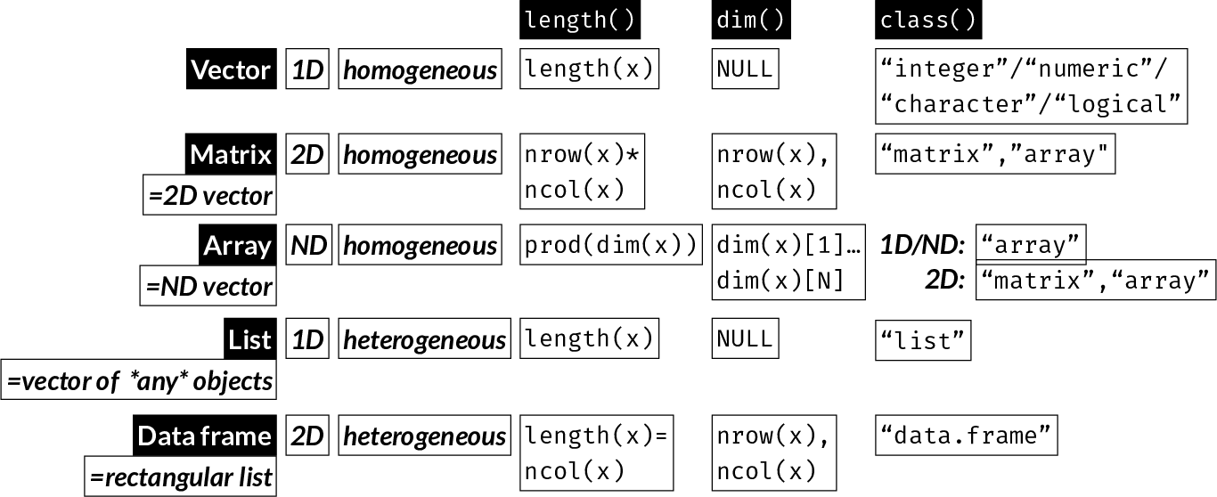
There are 5 main data structures in R:
| Data Structure | Dimensionality | Contents | Notes |
|---|---|---|---|
| Vector | 1D | homogeneous | the “base” object |
| Matrix | 2D | homogeneous | a vector with 2 dimensions |
| Array | ND | homogeneous | a vector with N dimensions |
| List | 1D; can be nested | heterogeneous | a collection of any R objects, each of any length |
| Data frame | 2D | heterogeneous | a special kind of list: a collection of (column) vectors of any type, all of the same length |
Vectors are homogeneous data structures which means all of their elements have to be of the same type (see Chapter 9), e.g. integer, double, character, logical.
Matrices and arrays are vectors with more dimensions, and as such, are also homogeneous.
Lists are the most flexible. Their elements can be any R objects, including lists, and therefore can be nested.
Data frames are a special kind of list. Their elements are one or more vectors, which can be of any type, and form columns. Therefore a data.frame is a two-dimensional data structure where rows typically correspond to cases (e.g. individuals) and columns represent variables. As such, data.frames are the most common data structure for statistical analysis.
10.2 Vectors
A vector is the most basic and fundamental data structure in R. Other data structures are made up of one or more vectors.
A vector has length() but no dim(), e.g.
10.2.1 Initializing a vector
10.3 Matrices
A matrix is a vector with 2 dimensions.
To create a matrix, you pass a vector to the matrix() function and specify number of rows using nrow and/or number of columns using ncol;
x <- matrix(21:50,
            nrow = 10, ncol = 3)
x
[,1] [,2] [,3]
[1,] 21 31 41
[2,] 22 32 42
[3,] 23 33 43
[4,] 24 34 44
[5,] 25 35 45
[6,] 26 36 46
[7,] 27 37 47
[8,] 28 38 48
[9,] 29 39 49
[10,] 30 40 50class(x)[1] "matrix" "array" A matrix has length (length(x)) equal to the number of all (i, j) elements or nrow * ncol (if i is the row index and j is the column index) and dimensions (dim(x)) as expected:
10.3.1 Construct by row vs. by column
By default, vectors are constructed by column (byrow = FALSE), e.g.
x <- matrix(1:20, nrow = 10, ncol = 2, byrow = FALSE)
x
[,1] [,2]
[1,] 1 11
[2,] 2 12
[3,] 3 13
[4,] 4 14
[5,] 5 15
[6,] 6 16
[7,] 7 17
[8,] 8 18
[9,] 9 19
[10,] 10 20You can set the byrow argument to TRUE to fill the matrix by row instead:
x <- matrix(1:20, nrow = 10, ncol = 2, byrow = TRUE)
x
[,1] [,2]
[1,] 1 2
[2,] 3 4
[3,] 5 6
[4,] 7 8
[5,] 9 10
[6,] 11 12
[7,] 13 14
[8,] 15 16
[9,] 17 18
[10,] 19 2010.3.2 Initialize a matrix
You can initialize a matrix with some constant value, e.g. 0:
x <- matrix(0, nrow = 6, ncol = 4)
x
[,1] [,2] [,3] [,4]
[1,] 0 0 0 0
[2,] 0 0 0 0
[3,] 0 0 0 0
[4,] 0 0 0 0
[5,] 0 0 0 0
[6,] 0 0 0 0To initialize a matrix with NA values, it is most efficient to use NA of the appropriate type, e.g. NA_real_ for a numeric matrix, NA_character_ for a character matrix, etc. See NA types.
For example, to initialize a numeric matrix with NA values:
x <- matrix(NA_real_, nrow = 6, ncol = 4)
x
[,1] [,2] [,3] [,4]
[1,] NA NA NA NA
[2,] NA NA NA NA
[3,] NA NA NA NA
[4,] NA NA NA NA
[5,] NA NA NA NA
[6,] NA NA NA NA10.3.3 Bind vectors by column or by row
Use cbind (“column-bind”) to convert a set of input vectors to columns of a matrix. The vectors must be of the same length:
x <- cbind(1:10, 11:20, 41:50)
x
[,1] [,2] [,3]
[1,] 1 11 41
[2,] 2 12 42
[3,] 3 13 43
[4,] 4 14 44
[5,] 5 15 45
[6,] 6 16 46
[7,] 7 17 47
[8,] 8 18 48
[9,] 9 19 49
[10,] 10 20 50class(x)[1] "matrix" "array" Similarly, you can use rbind (“row-bind”) to convert a set of input vectors to rows of a matrix. The vectors again must be of the same length:
10.3.4 Combine matrices
cbind() and rbind() can be used to combine two or more matrices together - or vector and matrices:
10.4 Arrays
Arrays are vectors with dimensions.
You can have 1D, 2D or any number of dimensions, i.e. ND arrays.
10.4.1 One-dimensional (“1D”) array
A 1D array is just like a vector but of class array and with dim(x) equal to length(x). Remember, vectors have only length(x) and undefined dim(x).
[1] "integer"is.vector(x)[1] TRUElength(x)[1] 10dim(x)NULLclass(xa)[1] "array"is.vector(xa)[1] FALSElength(xa)[1] 10dim(xa)[1] 10It is rather unlikely you will need to use a 1D array instead of a vector.
10.4.2 Two-dimensional (“2D”) array
A 2D array is a matrix:
10.4.3 Multi-dimensional (“ND”) array
You can build an N-dimensional array:
, , 1

     [,1] [,2] [,3] [,4]
[1,]    1    6   11   16
[2,]    2    7   12   17
[3,]    3    8   13   18
[4,]    4    9   14   19
[5,]    5   10   15   20

, , 2

     [,1] [,2] [,3] [,4]
[1,]   21   26   31   36
[2,]   22   27   32   37
[3,]   23   28   33   38
[4,]   24   29   34   39
[5,]   25   30   35   40

, , 3

     [,1] [,2] [,3] [,4]
[1,]   41   46   51   56
[2,]   42   47   52   57
[3,]   43   48   53   58
[4,]   44   49   54   59
[5,] 45 50 55 60class(x)[1] "array"You can provide names for each dimensions using the dimnames argument. It accepts a list where each elements is a character vector of length equal to the dimension length. Using the same example as above, we pass three character vector of length 5, 4, and 3 to match the length of the dimensions:
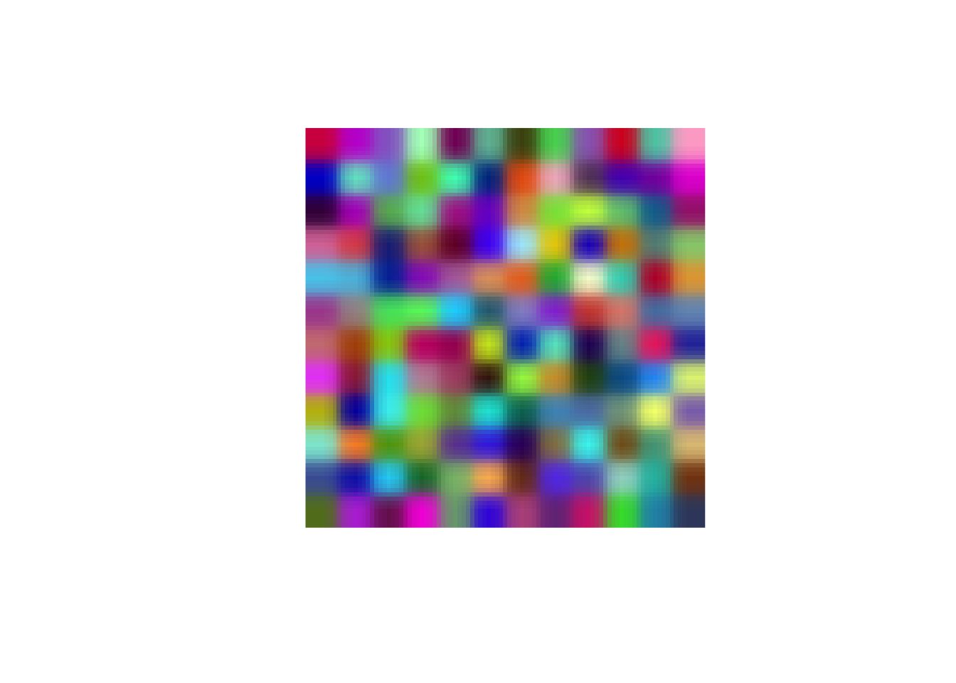
3D arrays can be used to represent color images. Here, just for fun, we use rasterImage() to show how you would visualize such an image:
10.5 Lists
To define a list, we use list() to pass any number of objects.
If these objects are passed as named arguments, the names will be used as element names:
[1] "list"str(x)List of 4
$ one : int [1:4] 1 2 3 4
$ two : num [1:10] 22.2 29.7 7.1 25.3 4 77 92.2 55.8 70.1 19.3
$ three: chr [1:3] "mango" "banana" "tangerine"
$ four :function (x, na.rm = FALSE, ...) length(x)[1] 410.5.1 Nested lists
Since each element can be any object, we can build nested lists:
$alpha
[1] "m" "v" "i" "s"

$beta
 [1]  6  9 11  7 12  1  3  2  5  8 10  4

$gamma
$gamma$i
 [1]  0.53247529  1.04208885  0.79405090  0.90198403  0.93227829 -0.37353712
 [7]  0.23329173 -0.18280114  0.01755548 -0.60783391

$gamma$j
 [1] 0.75520661 0.29037826 0.62411677 0.28914929 0.84581563 0.37069222
 [7] 0.84530931 0.29611865 0.50588479 0.07376151

$gamma$k
 [1]    0.0000  111.1111  222.2222  333.3333  444.4444  555.5556  666.6667
 [8]  777.7778  888.8889 1000.0000
In the example above, alpha, beta, and gamma, are x’s elements. Notice how the length of the list refers to the number of these top-level elements:
length(x)[1] 310.5.2 Initialize a list
When setting up experiments, it can be very convenient to set up and empty list, where results will be stored (e.g. using a for-loop):
10.5.3 Add element to a list
You can add a new elements to a list by assigning directly to an element that doesn’t yet exist, which will cause it to be created:
$a
 [1]  1  2  3  4  5  6  7  8  9 10

$b
 [1]  1.50982472 -0.44446244 -0.06501572  0.68257515  1.59842311  0.13404179
[7] -1.19596622 -2.30800762 1.65034654 -0.19447661x$c <- 30:21
x$a
[1] 1 2 3 4 5 6 7 8 9 10
$b
[1] 1.50982472 -0.44446244 -0.06501572 0.68257515 1.59842311 0.13404179
[7] -1.19596622 -2.30800762 1.65034654 -0.19447661
$c
[1] 30 29 28 27 26 25 24 23 22 2110.5.4 Combine lists
You can combine lists with c(), just like vectors:
10.6 Combining different types with c()
It’s best to use c() to either combine elements of the same type into a vector, or to combine lists.
As we’ve seen, if all arguments passed to c() are of a single type, you get a vector of that type:
If arguments passed to c() are a mix of numeric and character, they all get coerced to character.
If you pass more types of objects (which cannot be coerced to character) you get a list, since it is the only structure that can support all of them together:
10.7 Data frames
A data frames is a special type of list where each element has the same length and forms a column, resulting in a 2D structure. Unlike matrices, each column can contain a different data type.
data.frames are usually created with named elements:
x <- data.frame(Feat_1 = 1:5,
                Feat_2 = rnorm(5),
                Feat_3 = paste0("rnd_", sample(seq(100), size = 5)))
x
Feat_1 Feat_2 Feat_3
1 1 -0.2025701 rnd_44
2 2 -0.3018923 rnd_61
3 3 -0.7525255 rnd_99
4 4 0.6674210 rnd_78
5 5 -1.4970134 rnd_14class(x)[1] "data.frame"str(x)'data.frame': 5 obs. of 3 variables:
$ Feat_1: int 1 2 3 4 5
$ Feat_2: num -0.203 -0.302 -0.753 0.667 -1.497
$ Feat_3: chr "rnd_44" "rnd_61" "rnd_99" "rnd_78" ...class(x$Feat_1)[1] "integer"Unlike a matrix, the elements of a data.frame are its columns, not the individual values in each position. Therefore the length of a data.frame is equal to the number of columns.
Just like with lists, you can add new columns to a data.frame using assignment to a new element, i.e. column:
x <- data.frame(PIDN = sample(8001:9000, size = 10, replace = TRUE),
                Age = rnorm(10, mean = 48, sd = 2.9))
x
PIDN Age
1 8393 43.08571
2 8672 46.28453
3 8231 50.01578
4 8390 45.98363
5 8210 41.96492
6 8771 50.63188
7 8443 47.21445
8 8783 53.40193
9 8926 48.97619
10 8606 43.43932x$Weight <- rnorm(10, mean = 84, sd = 1.5)
x PIDN Age Weight
1 8393 43.08571 83.79544
2 8672 46.28453 83.89163
3 8231 50.01578 82.15262
4 8390 45.98363 86.62266
5 8210 41.96492 83.62964
6 8771 50.63188 84.69530
7 8443 47.21445 83.91734
8 8783 53.40193 85.57177
9 8926 48.97619 83.75611
10 8606 43.43932 83.2175110.8 Generating sequences
Other than assigning individual elements explicitly with c(), there are multiple ways to create numeric sequences.
Colon notation allows generating a simple integer sequence:
seq(from, to, by)
seq(1, 10, by = 0.5) [1] 1.0 1.5 2.0 2.5 3.0 3.5 4.0 4.5 5.0 5.5 6.0 6.5 7.0 7.5 8.0
[16] 8.5 9.0 9.5 10.0seq(from, to, length.out = n)
seq(-5, 12, length.out = 11) [1] -5.0 -3.3 -1.6 0.1 1.8 3.5 5.2 6.9 8.6 10.3 12.0seq(object) generates a sequence of length equal to length(object)
seq(iris)[1] 1 2 3 4 5seq_along(object) is the optimized version of seq(object):
seq_along(iris)[1] 1 2 3 4 5seq(n) is equivalent to 1:n
seq_len(n) is an optimized version of seq(n):
seq_len(12) [1] 1 2 3 4 5 6 7 8 9 10 11 1210.9 Naming object elements
All objects’ elements can be named.
10.9.1 Vectors
You can create a vector with named elements:
SBP = c(before = 179, after = 118)
SBP
before after
179 118 Use names() to get a vector’s elements’ names:
names(SBP)[1] "before" "after" You can add names to an existing, unnamed, vector:
Matrices and data frames can have column names (colnames) and row names (rownames):
xm <- matrix(1:15, nrow = 5)
xdf <- as.data.frame(xm)
colnames(xm)NULLcolnames(xdf)[1] "V1" "V2" "V3"rownames(xm)NULL Feature1 Feature2 Feature3
Case1 1 6 11
Case2 2 7 12
Case3 3 8 13
Case4 4 9 14
Case5 5 10 15xdf Feature1 Feature2 Feature3
Case1 1 6 11
Case2 2 7 12
Case3 3 8 13
Case4 4 9 14
Case5 5 10 15Lists are vectors so they have names. These can be defined when a list is created using the name-value pairs or added/changed at any time.
[1] "HospitalName"             "ParticipatingDepartments"
[3] "PatientIDs"
Add/Change names:
$Hospital
[1] "CaliforniaGeneral"

$Departments
[1] "Neurology"    "Psychiatry"   "Neurosurgery"

$PIDs
 [1] 1001 1002 1003 1004 1005 1006 1007 1008 1009 1010 1011 1012 1013 1014 1015
[16] 1016 1017 1018
Remember that data a frame is a special type of list. Therefore in data frames colnames and names are equivalent:
colnames(iris)[1] "Sepal.Length" "Sepal.Width" "Petal.Length" "Petal.Width" "Species" names(iris)[1] "Sepal.Length" "Sepal.Width" "Petal.Length" "Petal.Width" "Species" Note: As we saw, matrices have colnames() and rownames() Using names() on a matrix will assign names to individual elements, as if it was a long vector.
10.10 Initialize - coerce - test data structures
The following table lists the functions to initialize, coerce (=convert), and test the core data structures, which are shown in more detail in the following paragraphs:
| Initialize | Coerce | Test |
|---|---|---|
matrix(NA, nrow = x, ncol = y) |
as.matrix(x) |
is.matrix(x) |
array(NA, dim = c(x, y, z)) |
as.array(x) |
is.array(x) |
vector(mode = "list", length = x) |
as.list(x) |
is.list(x) |
data.frame(matrix(NA, x, y)) |
as.data.frame(x) |
is.data.frame(x) |
10.11 Attributes
R objects may have some builtin attributes but you can add arbitrary attributes to any R object. These are used to store additional information, sometimes called metadata.
10.11.1 Print all attributes
To print an object’s attributes, use attributes:
attributes(iris)$names
[1] "Sepal.Length" "Sepal.Width" "Petal.Length" "Petal.Width" "Species"
$class
[1] "data.frame"
$row.names
[1] 1 2 3 4 5 6 7 8 9 10 11 12 13 14 15 16 17 18
[19] 19 20 21 22 23 24 25 26 27 28 29 30 31 32 33 34 35 36
[37] 37 38 39 40 41 42 43 44 45 46 47 48 49 50 51 52 53 54
[55] 55 56 57 58 59 60 61 62 63 64 65 66 67 68 69 70 71 72
[73] 73 74 75 76 77 78 79 80 81 82 83 84 85 86 87 88 89 90
[91] 91 92 93 94 95 96 97 98 99 100 101 102 103 104 105 106 107 108
[109] 109 110 111 112 113 114 115 116 117 118 119 120 121 122 123 124 125 126
[127] 127 128 129 130 131 132 133 134 135 136 137 138 139 140 141 142 143 144
[145] 145 146 147 148 149 150This returns a named list. In this case we got names, class, and row.names of the iris data frame.
10.11.2 Get or set specific attributes
You can assign new attributes using attr:
Printing the vector after adding a new attribute, prints the attribute name and value underneath the vector itself:
x [1] 1 2 3 4 5 6 7 8 9 10
attr(,"name")
[1] "Very special vector"Our trusty str function will print attributes as well:
str(x) int [1:10] 1 2 3 4 5 6 7 8 9 10
- attr(*, "name")= chr "Very special vector"10.11.2.1 A matrix is a vector - a closer look
Let’s see how a matrix is literally just a vector with assigned dimensions.
Start with a vector of length 20:
x <- 1:20
x
[1] 1 2 3 4 5 6 7 8 9 10 11 12 13 14 15 16 17 18 19 20The vector has no attributes - yet:
attributes(x)NULLTo convert to a matrix, we would normally pass our vector to the matrix() function and define number of rows and/or columns:
xm <- matrix(x, nrow = 5)
xm
[,1] [,2] [,3] [,4]
[1,] 1 6 11 16
[2,] 2 7 12 17
[3,] 3 8 13 18
[4,] 4 9 14 19
[5,] 5 10 15 20attributes(xm)$dim
[1] 5 4Just for demonstration, let’s instead directly add a dimension attribute to our vector:
     [,1] [,2] [,3] [,4]
[1,]    1    6   11   16
[2,]    2    7   12   17
[3,]    3    8   13   18
[4,]    4    9   14   19
[5,] 5 10 15 20class(x)[1] "matrix" "array" Just like that, we have created a matrix.
10.12 Further study
Optional reading:
- PDSR: Data Structures — Source chapter and continuing reference.
- PDSR: Data frame basics — Further operations on tabular data.